1 SIRS Model
The
SIRS model is simply an extension of the
SIR model as it allows members of the recovered class to rejoin the susceptible class at a defined rate, which integrates the impact of waning immunity following antigenic drift. Similar to the SIR model, a fixed population without births and deaths is considered in the SIRS model. The standard form of SIRS model is described as
$$
\begin{equation}
\begin{aligned}
& \frac{dS}{dt} = fR - \frac{\beta SI}{N} \\
& \frac{dI}{dt} = \frac{\beta SI}{N} - \gamma I \\
& \frac{dR}{dt} = \gamma I - fR
\end{aligned}
\label{eq1}
\end{equation}
$$
where \(f\) is the average loss of immunity rate of recovered indiviuals, and the other notations are the same as the SIR model. Note that SIR model is a special case of SIRS model under condition of \(f = 0\). Hence, it is possible to create a general function to solve both SIR and SIRS models.
As only two of the three ODEs are independent, \(R(t)\) does not have to be treated explicitly and using ODEs of \(S(t)\) and \(I(t)\) to describe the dynamic of SIRS model are adequate. Substitute \(R(t) = N - S(t) - I(t)\) into ODE of \(S(t)\) and the formula is simplified as follows
$$
\begin{equation}
\begin{aligned}
& \frac{dS}{dt} = f(N - S - I) - \frac{\beta SI}{N} \\
& \frac{dI}{dt} = \frac{\beta SI}{N} - \gamma I
\end{aligned}
\label{eq2}
\end{equation}
$$
The form of SIRS model described in
Dushoff et al. (2004) and
Shaman et al. (2010) is as follows
$$
\begin{equation}
\begin{aligned} \label{eq3}
& \frac{dS}{dt} = \frac{N - S - I}{L} - \frac{\beta SI}{N} \\
& \frac{dI}{dt} = \frac{\beta SI}{N} - \frac{I}{D}
\end{aligned}
\end{equation}
$$
where \(L\) is the average duration of immunity of recoverd indiviuals, and \(D\) is the mean infectious period of infected indiviuals. Comparing with ODEs \((\ref{eq2})\), \(L = \frac{1}{f}\) and \(D = \frac{1}{\gamma}\) are derived.
In the following subsections, RK4 method is applied to solve SIRS model in different forms.
1.1 RK4SIRS.std function
The iterative formula of RK4 method for solving SIRS model in the standard form \((\ref{eq1})\) can be easily derived and won’t be presented here. The following codes firstly define four helper functions. Three of them describe \(S(t)\), \(I(t)\) and \(R(t)\) compartments of SIRS model. The other one defines the infection rate (see Table 1 in
Dushoff et al. (2004)) to calculate cummulative incidence. Different from SIR model, the infection rate is only the second term of \(S(t)\) compartment in SIRS model. Therefore, an additional helper function is needed to separately define the infection rate.
# define S, I, R compartments of SIRS model
dSdt.std <- function(t, S, I, R) {
  return(f * R - beta * S * I / N)
}

dIdt.std <- function(t, S, I) {
  return(beta * S * I / N - gamma * I)
}

dRdt.std <- function(t, I, R) {
  return(gamma * I - f * R)
}

# define infection rate
dCIdt.std <- function(t, S, I) {
  return(beta * S * I / N)
}
The iterative algorithm for calculating cummumcaltive incidence resembles those of \(S(t)\), \(I(t)\) and \(R(t)\). The implementation of RK4 method for SIRS model is presented as follows.
# RK4 method for the numerical integration of SIRS model in standard form
RK4SIRS.std <- function(n, beta, gamma, f, S0, I0, R0 = 0, dt = 1, incidence = FALSE) {
  N <<- S0 + I0 + R0

  S <- c(S0, rep(0, n))
  I <- c(I0, rep(0, n))
  R <- c(R0, rep(0, n))
  CI <- c(I0, rep(0, n))  # cummulative incidence
  for (i in 1:n) {
    Si <- S[i]
    Ii <- I[i]
    Ri <- R[i]
    CIi <- CI[i]

    S.k1 <- dSdt.std(i, Si, Ii, Ri)
    I.k1 <- dIdt.std(i, Si, Ii)
    R.k1 <- dRdt.std(i, Ii, Ri)
    CI.k1 <- dCIdt.std(i, Si, Ii)

    S.k2 <- dSdt.std(i + dt / 2, Si + dt / 2 * S.k1, Ii + dt / 2 * I.k1, Ri + dt / 2 * R.k1)
    I.k2 <- dIdt.std(i + dt / 2, Si + dt / 2 * S.k1, Ii + dt / 2 * I.k1)
    R.k2 <- dRdt.std(i + dt / 2, Ii + dt / 2 * I.k1, Ri + dt / 2 * R.k1)
    CI.k2 <- dCIdt.std(i + dt / 2, Si + dt / 2 * S.k1, Ii + dt / 2 * I.k1)

    S.k3 <- dSdt.std(i + dt / 2, Si + dt / 2 * S.k2, Ii + dt / 2 * I.k2, Ri + dt / 2 * R.k2)
    I.k3 <- dIdt.std(i + dt / 2, Si + dt / 2 * S.k2, Ii + dt / 2 * I.k2)
    R.k3 <- dRdt.std(i + dt / 2, Ii + dt / 2 * I.k2, Ri + dt / 2 * R.k2)
    CI.k3 <- dCIdt.std(i + dt / 2, Si + dt / 2 * S.k2, Ii + dt / 2 * I.k2)

    S.k4 <- dSdt.std(i + dt, Si + dt * S.k3, Ii + dt * I.k3, Ri + dt * R.k3)
    I.k4 <- dIdt.std(i + dt, Si + dt * S.k3, Ii + dt * I.k3)
    R.k4 <- dRdt.std(i + dt, Ii + dt * I.k3, Ri + dt * R.k3)
    CI.k4 <- dCIdt.std(i + dt, Si + dt * S.k3, Ii + dt * I.k3)

    S[i + 1] <- Si + dt / 6 * (S.k1 + 2 * S.k2 + 2 * S.k3 + S.k4)
    I[i + 1] <- Ii + dt / 6 * (I.k1 + 2 * I.k2 + 2 * I.k3 + I.k4)
    R[i + 1] <- Ri + dt / 6 * (R.k1 + 2 * R.k2 + 2 * R.k3 + R.k4)
    CI[i + 1] <- CIi + dt / 6 * (CI.k1 + 2 * CI.k2 + 2 * CI.k3 + CI.k4)
  }
  if (!incidence) {
    return(data.frame(n = 0:n, S = S, I = I, R = R))
  } else {
    # newly infected per day (incidence)
    inc = c(I0, diff(CI))
    return(data.frame(n = 0:n, S = S, I = I, R = R, inc = inc, cum.inc = CI))
  }
}
1.2 RK4SIRS function
There are many repetitive computations in the implementation of RK4SIRS.std function, especially for calculating cummulative incidence. Actually, the system of ODEs of SIRS model describes the transition of an individual between susceptible, infectious, and recovered states. For SIRS model in simplified form \((\ref{eq2})\), only susceptible and infectious states are necessary to represent the system state and the system state at time \(t\) is usually expressed as state vector \(\mathbf{Z}(t)\equiv (S(t), I(t))\). As presented in Table 1, infection, recovery, and immunity loss events can change the system state at a rate of \(\frac{\beta SI}{N}\), \(\gamma I\), and \(f(N-S-I)\), respectively.
Table: Table 1. Markov chain transition rate (source: Dushoff et al. (2004))
Event Change Rate
Infection \((S,I)\rightarrow (S-1,I+1)\) \(\frac{\beta SI}{N}\)
Recovery \((S,I)\rightarrow (S, I-1)\) \(\gamma I\)
Immunity loss \((S,I)\rightarrow (S+1, I)\) \(f(N-S-I)\)
Instead of directly defining \(S(t)\) and \(I(t)\) compartments of SIRS model, using helper functions to define the events can avoid redundant computing as events describe the changes in system state at fine-grained scale. According to Table 1, RK4 method for solving SIRS model in simplified form \((\ref{eq2})\) can be easily implemented by slightly modified from RK4SIRS.std function.
# define infection rate
inf.rate <- function(t, S, I) {
  return(beta * S * I / N)
}

# define recovery rate
rec.rate <- function(t, I) {
  return(gamma * I)
}

# define immunity loss rate
ilos.rate <- function(t, S, I) {
  return(f * (N - S - I))
}

# RK4 method for numerical integration of SIRS model in simplified form
RK4SIRS <- function(n, beta, gamma, f, S0, I0, R0 = 0, dt = 1, incidence = FALSE) {
  N <<- S0 + I0 + R0

  S <- c(S0, rep(0, n))
  I <- c(I0, rep(0, n))
  R <- c(R0, rep(0, n))
  CI <- c(I0, rep(0, n))  # cummulative incidence
  for (i in 1:n) {
    Si <- S[i]
    Ii <- I[i]
    Ri <- R[i]
    CIi <- CI[i]

    Einf <- inf.rate(i, Si, Ii)  # event of infection
    Erec <- rec.rate(i, Ii)  # event of recovery
    Eilos <- ilos.rate(i, Si, Ii)  # event of immunity loss
    S.k1 <- Eilos - Einf
    I.k1 <- Einf - Erec
    CI.k1 <- Einf

    Einf <- inf.rate(i + dt / 2, Si + dt / 2 * S.k1, Ii + dt / 2 * I.k1)
    Erec <- rec.rate(i + dt / 2, Ii + dt / 2 * I.k1)
    Eilos <- ilos.rate(i + dt / 2, Si + dt / 2 * S.k1, Ii + dt / 2 * I.k1)
    S.k2 <- Eilos - Einf
    I.k2 <- Einf - Erec
    CI.k2 <- Einf

    Einf <- inf.rate(i + dt / 2, Si + dt / 2 * S.k2, Ii + dt / 2 * I.k2)
    Erec <- rec.rate(i + dt / 2, Ii + dt / 2 * I.k2)
    Eilos <- ilos.rate(i + dt / 2, Si + dt / 2 * S.k2, Ii + dt / 2 * I.k2)
    S.k3 <- Eilos - Einf
    I.k3 <- Einf - Erec
    CI.k3 <- Einf

    Einf <- inf.rate(i + dt, Si + dt * S.k3, Ii + dt * I.k3)
    Erec <- rec.rate(i + dt, Ii + dt * I.k3)
    Eilos <- ilos.rate(i + dt, Si + dt * S.k3, Ii + dt * I.k3)
    S.k4 <- Eilos - Einf
    I.k4 <- Einf - Erec
    CI.k4 <- Einf

    S[i + 1] <- Si + dt / 6 * (S.k1 + 2 * S.k2 + 2 * S.k3 + S.k4)
    I[i + 1] <- Ii + dt / 6 * (I.k1 + 2 * I.k2 + 2 * I.k3 + I.k4)
    CI[i + 1] <- CIi + dt / 6 * (CI.k1 + 2 * CI.k2 + 2 * CI.k3 + CI.k4)
  }
  R <- N - S - I

  if (!incidence) {
    return(data.frame(n = 0:n, S = S, I = I, R = R))
  } else {
    # newly infected per day (incidence)
    inc = c(I0, diff(CI))
    return(data.frame(n = 0:n, S = S, I = I, R = R, inc = inc, cum.inc = CI))
  }
}
1.3 rk4 function
Using rk4 function from deSolve package to solve SIRS model only needs to redefine the model and the vector of parameters used in SIRS model.
# vector of parameters used in SIRS model
params <- c(beta = beta, gamma = gamma, f = f)
# definition of SIRS model
SIRS <- function(t, y, params) {
  with(as.list(c(params, y)), {
    dS <- f * R - beta * S * I / N
    dI <- beta * S * I / N - gamma * I
    dR <- gamma * I - f * R
    list(c(dS, dI, dR))
  })
}
The above three functions are tested with the same study case of the spread of Hong Kong flu in New York city and they all give the same results. Note that the parameter \(f = \frac{1}{L} = \frac{1}{3.86 \times 365}\) comes from the parameters combination for generation of synthetic truth in
Shaman and Karspeck (2012). Here, only results given by RK4SIRS function are presented to avoid redundancy.
# simulate the spread of Hong Kong flu of NYC
S0 <- 7900000
I0 <- 10
beta <- 1 / 2
gamma <- 1 / 3  # gamma = 1 / D
f <- 1 / (3.86 * 365)  # L = 3.86 years, f = 1 / L
n <- 200

r <- RK4SIRS(n, beta, gamma, f, S0, I0, incidence = TRUE)
# plot S, I, R curves
library(reshape2)
r.plot <- melt(r, id = "n", measure = c("S", "I", "R", "inc", "cum.inc"))
library(ggplot2)
p <- ggplot(r.plot, aes(x = n, y = value, group = variable, color = variable))
p + geom_line() +
  scale_colour_discrete(name = "Legend",
                        breaks = c("S", "I", "R", "inc", "cum.inc"),
                        labels = c("Susceptible", "Infected ", "Recovered", "Incidence",
                                   "Cumulative incidence")) +
  ggtitle("Spread of Hong Kong Flu in New York City")
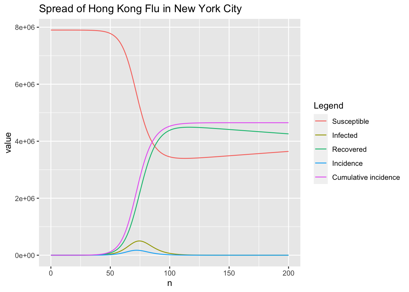
# peak of the infected
which.max(r$I)
## [1] 75
max(r$I)
## [1] 499451.1
# peak of incidence
which.max(r$inc)
## [1] 73
max(r$inc)
## [1] 174175.2
1.4 Benchmark
RK4SIRS.std, RK4SIRS and rk4 are separately runned 1000 times for benchmark performance analysis.
####
library(deSolve)
# initial (state) values for SIR model
y0 <- c(S = S0, I = I0, R = 0)
# vector of time steps
times <- 0:n
# vector of parameters used in SIRS model
params <- c(beta = beta, gamma = gamma, f = f)
# definition of SIRS model
SIRS <- function(t, y, params) {
  with(as.list(c(params, y)), {
    dS <- f * R - beta * S * I / N
    dI <- beta * S * I / N - gamma * I
    dR <- gamma * I - f * R
    list(c(dS, dI, dR))
  })
}
####
# benchmark
library(microbenchmark)
compare <- microbenchmark(rk4(y0, times, SIRS, params),
                          RK4SIRS(n, beta, gamma, f, S0, I0, incidence = TRUE),
                          RK4SIRS.std(n, beta, gamma, f, S0, I0, incidence = TRUE),
                          times = 10)
# change expr for display
compare$expr <- gsub("rk4(y0, times, SIRS, params)", "rk4",
                     compare$expr, fixed = TRUE)
compare$expr <- gsub("RK4SIRS(n, beta, gamma, f, S0, I0, incidence = TRUE)", "RK4SIRS",
                     compare$expr, fixed = TRUE)
compare$expr <- gsub("RK4SIRS.std(n, beta, gamma, f, S0, I0, incidence = TRUE)",
                     "RK4SIRS.std", compare$expr, fixed = TRUE)
compare
## Unit: milliseconds
##         expr      min        lq      mean    median        uq       max neval
##          rk4 11.46048 11.619344 13.132164 11.709227 12.170580 22.100666    10
##      RK4SIRS  2.66024  2.858313  3.158156  2.890771  2.994426  5.543579    10
##  RK4SIRS.std  4.17314  4.258929 13.824397  4.366474  4.504573 99.067068    10
# plot comparing results
library(ggplot2)
p <- autoplot(compare)
## Coordinate system already present. Adding new coordinate system, which will
## replace the existing one.
p + geom_violin(aes(color = expr, fill = expr)) +
  theme(legend.position = "none")
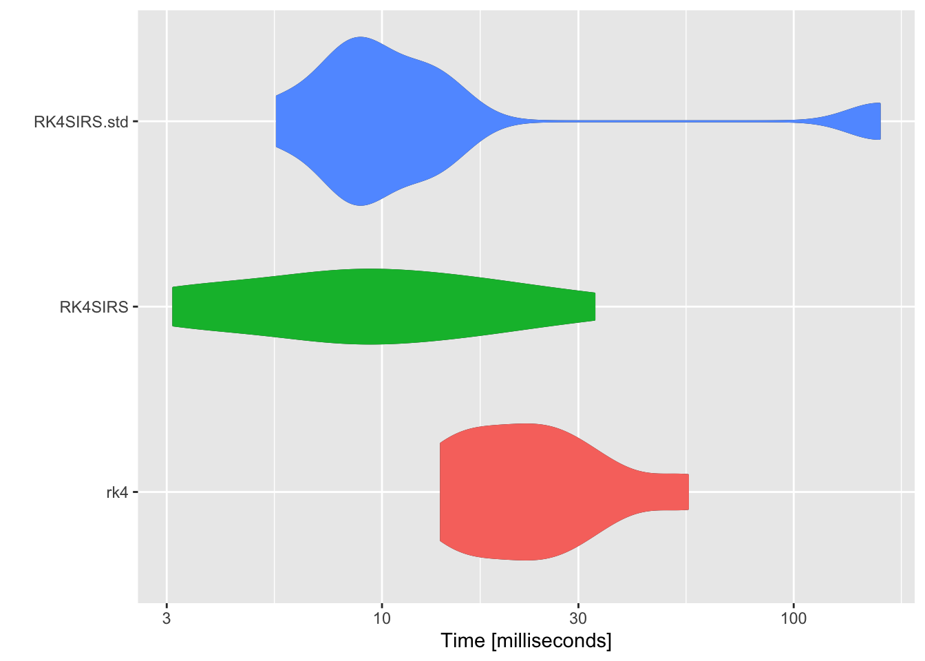
As shown in the above figure, RK4SIRS function runs the fastest. Subsequently, SIRS model will be solved in simplified form \eqref{eq:2}.
1.5 Basic Reproductive Number \(R_0\)
Technically, the
basic reproductive number \(R_0\) is defined as the number of secondary infections caused by a single infective introduced into a population made up entirely of susceptible individuals over the course of the infection of this single infective. For the susceptible population ($S_0 \approx N$), this infective individual makes \(\beta\) contacts per unit time producing new infections with a mean infectious period of \(D\). Therefore, the basic reproduction number is
$$
\begin{equation} \label{eq4}
R_0 = \beta D = \frac{\beta}{\gamma}
\end{equation}
$$
Actually, the basic reproductive number is often compared to 1 to determine whether an epidemic occurs or the disease simply dies out.
2 Time Dependent Transmission Rate \(\beta(t)\)
Equation (4) in
Shaman et al. (2010) shows the relationship between basic reproductive number \(R_0(t)\) and specific humidity \(q(t)\) at time \(t\). Combining with equation \((\ref{eq4})\), it’s easy to deduce that transmission rate \(\beta\) is also modulated by specific humidity \(q\) and time dependent. Hence, replacing the constant \(\beta\) in ODEs \((\ref{eq2})\) with time dependent \(\beta (t)\) can make SIRS model more reasonable. The resulting SIRS model with time dependent transmission rate \(\beta (t)\) is expressed as follow
$$
\begin{equation}
\begin{aligned} \label{eq:5}
& \frac{dS}{dt} = f(N - S - I) - \frac{\beta (t) SI}{N} \\
& \frac{dI}{dt} = \frac{\beta (t) SI}{N} - \gamma I
\end{aligned}
\end{equation}
$$
2.1 Implementation
The RK4 method for numerical integration of SIRS model with time dependent transmission rate \(\beta(t)\) can be easily implemented by adding parameters to helper event functions.
# define infection rate
inf.rate <- function(t, beta, S, I) {
  return(beta * S * I / N)
}

# define recovery rate
rec.rate <- function(t, gamma, I) {
  return(gamma * I)
}

# define immunity loss rate
ilos.rate <- function(t, f, S, I) {
  return(f * (N - S - I))
}

# beta is a numeric vector of length n or 1
RK4SIRS <- function(n, beta, gamma, f, S0, I0, R0 = 0, dt = 1, incidence = FALSE) {
  N <<- S0 + I0 + R0

  S <- c(S0, rep(0, n))
  I <- c(I0, rep(0, n))
  R <- c(R0, rep(0, n))
  CI <- c(I0, rep(0, n))  # cummulative incidence
  for (i in 1:n) {
    bti <- beta[i]
    Si <- S[i]
    Ii <- I[i]
    CIi <- CI[i]

    Einf <- inf.rate(i, bti, Si, Ii)  # event of infection
    Erec <- rec.rate(i, gamma, Ii)  # event of recovery
    Eilos <- ilos.rate(i, f, Si, Ii)  # event of immunity loss
    S.k1 <- Eilos - Einf
    I.k1 <- Einf - Erec
    CI.k1 <- Einf

    Einf <- inf.rate(i + dt / 2, bti, Si + dt / 2 * S.k1, Ii + dt / 2 * I.k1)
    Erec <- rec.rate(i + dt / 2, gamma, Ii + dt / 2 * I.k1)
    Eilos <- ilos.rate(i + dt / 2, f, Si + dt / 2 * S.k1, Ii + dt / 2 * I.k1)
    S.k2 <- Eilos - Einf
    I.k2 <- Einf - Erec
    CI.k2 <- Einf

    Einf <- inf.rate(i + dt / 2, bti, Si + dt / 2 * S.k2, Ii + dt / 2 * I.k2)
    Erec <- rec.rate(i + dt / 2, gamma, Ii + dt / 2 * I.k2)
    Eilos <- ilos.rate(i + dt / 2, f, Si + dt / 2 * S.k2, Ii + dt / 2 * I.k2)
    S.k3 <- Eilos - Einf
    I.k3 <- Einf - Erec
    CI.k3 <- Einf

    Einf <- inf.rate(i + dt, bti, Si + dt * S.k3, Ii + dt * I.k3)
    Erec <- rec.rate(i + dt, gamma, Ii + dt * I.k3)
    Eilos <- ilos.rate(i + dt, f, Si + dt * S.k3, Ii + dt * I.k3)
    S.k4 <- Eilos - Einf
    I.k4 <- Einf - Erec
    CI.k4 <- Einf

    S[i + 1] <- Si + dt / 6 * (S.k1 + 2 * S.k2 + 2 * S.k3 + S.k4)
    I[i + 1] <- Ii + dt / 6 * (I.k1 + 2 * I.k2 + 2 * I.k3 + I.k4)
    CI[i + 1] <- CIi + dt / 6 * (CI.k1 + 2 * CI.k2 + 2 * CI.k3 + CI.k4)
  }
  R <- N - S - I

  if (!incidence) {
    return(data.frame(n = 0:n, S = S, I = I, R = R))
  } else {
    # newly infected per day (incidence)
    inc = c(I0, diff(CI))
    return(data.frame(n = 0:n, S = S, I = I, R = R, inc = inc, cum.inc = CI))
  }
}
2.2 Simulation
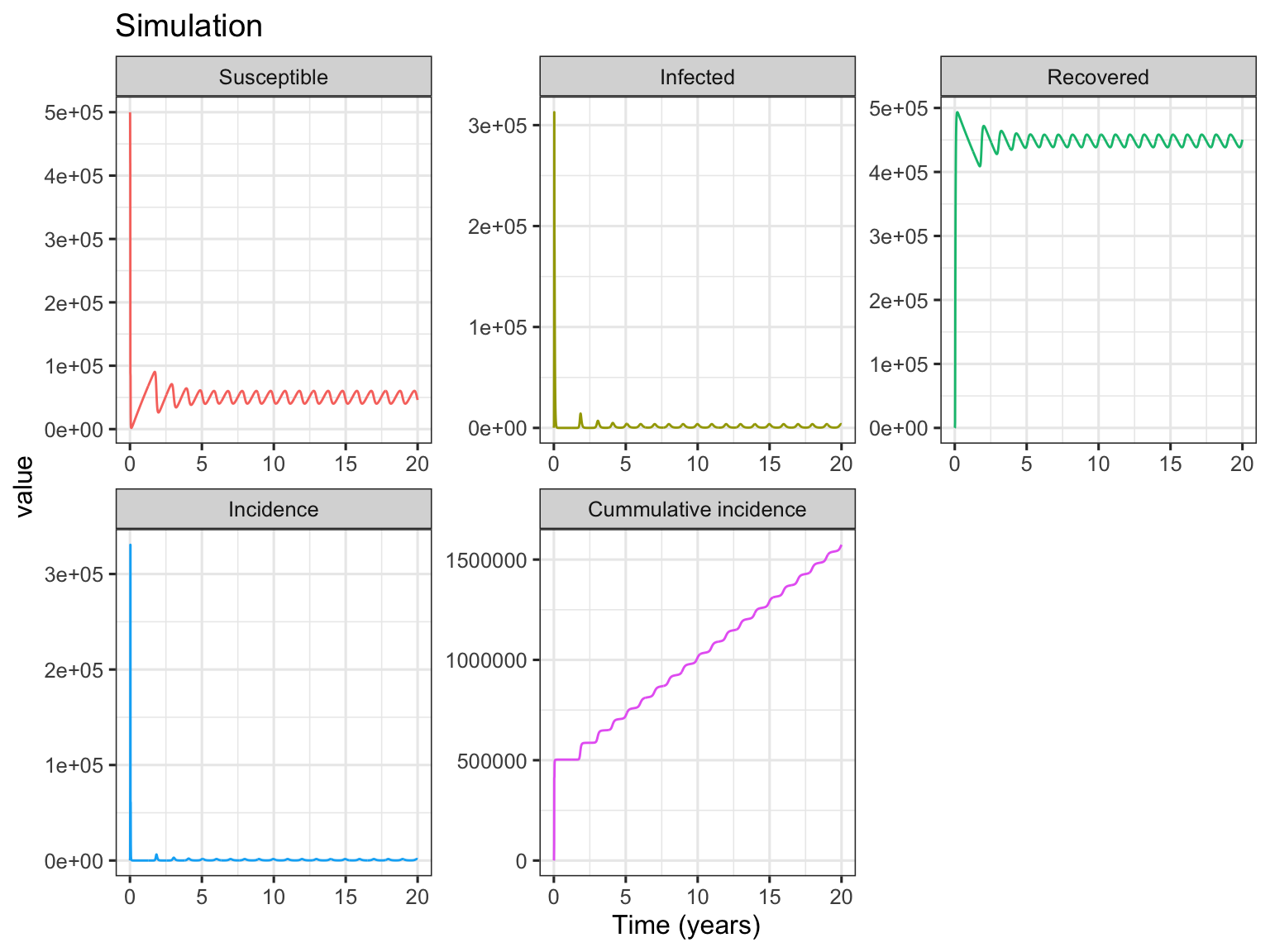
The following simulation example is adapted from Fig. 1a in Dushoff et al. (2004).
S0 <- 500000
I0 <- 100  # I0 has little effect on the dynamic equilibrium
R0 <- 0
N <- S0 + I0 + R0
L <- 4  # yr
f <- 1 / L
D <- 0.02  # yr
gamma <- 1 / D
dt <- 0.01  # yr
t <- seq(from = 0, to = 20, by = dt)
beta0 <- 500  # persons per yr
beta1 <- 0.04
beta <- beta0 * (1 + beta1 * cos(2 * pi * t))
n <- length(t[-1])

r <- RK4SIRS(n, beta, gamma, S0, I0, f = f, dt = dt, incidence = TRUE)
r <- cbind(t, r)
# plot S, I, R curves
library(reshape2)
r.plot <- melt(r, id = "t", measure = c("S", "I", "R", "inc", "cum.inc"))
# change levels for display
levels(r.plot$variable) <- c("Susceptible", "Infected", "Recovered", "Incidence",
                             "Cummulative incidence")
library(ggplot2)
p <- ggplot(r.plot, aes(x = t, y = value, group = variable, color = variable))
p + geom_line() +
  xlab("Time (years)") +
  facet_wrap(~ variable, scales = "free") +
  ggtitle("Simulation") +
  theme_bw(base_size = 12) +
  theme(legend.position = "none")
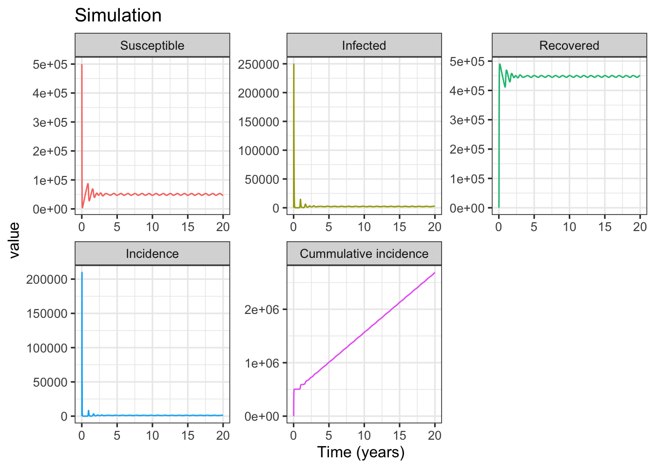
In Fig. 1a simulation, the basic reproductive number \(R_0=D\beta_0=\) 10, and the intrinsic period of oscillation \(T=2\pi \sqrt{\frac{DL}{R_0-1}}=\) 0.59. As shown in above figures, after starting simulation for several years, the compartments of SIRS model (including incidence) are in dynamic equilibrium. To show the details of deterministic equilibrium, the following codes only plot the subset results of 10 ~ 20 years.
r.eqb <- r[r$t >= 10, ]
r.plot <- melt(r.eqb, id = "t", measure = c("S", "I", "R", "inc", "cum.inc"))
levels(r.plot$variable) <- c("Susceptible", "Infected", "Recovered", "Incidence",
                             "Cummulative incidence")
p <- ggplot(r.plot, aes(x = t, y = value, group = variable, color = variable))
p + geom_line() +
  scale_x_continuous(breaks = 10:20, labels = 10:20, expand = c(0, 0)) +
  xlab("Time (years)") +
  facet_wrap(~ variable, scales = "free", ncol = 1) +
  ggtitle("Subset Results of Equilibrium") +
  theme_bw(base_size = 14) +
  theme(legend.position = "none")
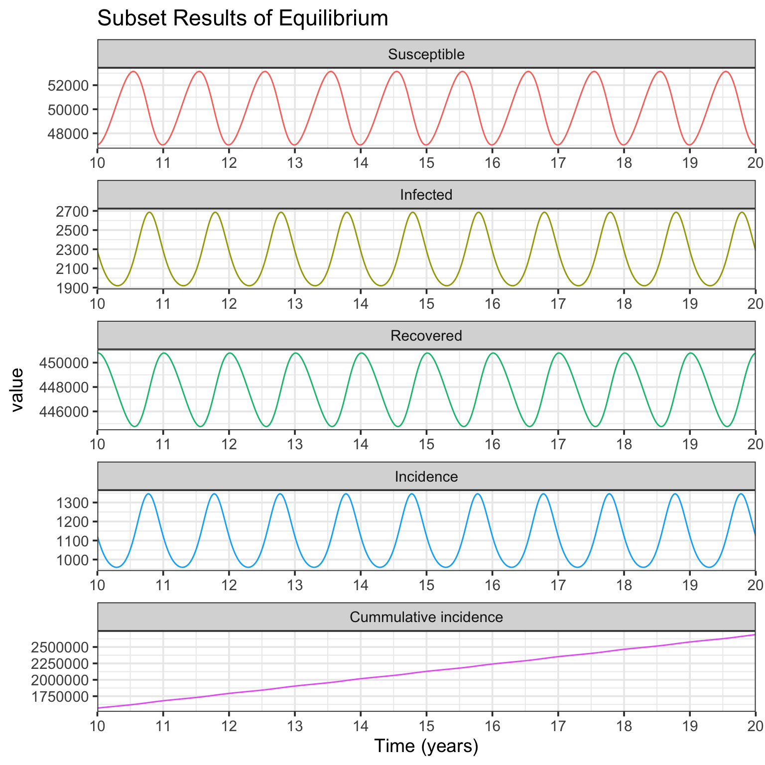
The Fig. 1b simulation is very similar to Fig. 1a, but with different parameters of \(L=8\) yr, \(D=0.025\) yr, and \(\beta_0=400\) persons per yr. The resulting plots of simulation are presented.
L <- 8  # yr
D <- 0.025  # yr
beta0 <- 400  # persons per yr
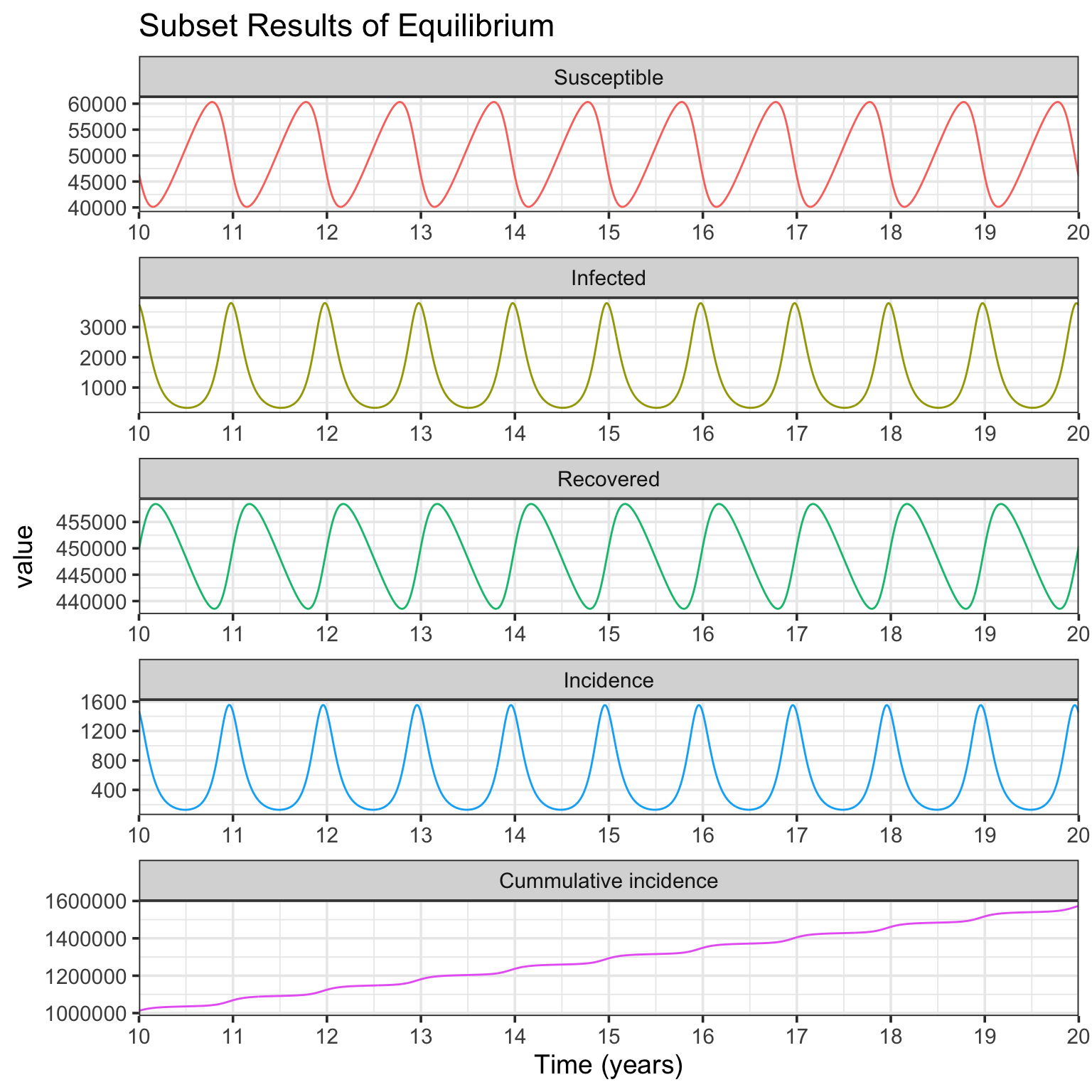
In Fig. 1b simulation, the basic reproductive number \(R_0=\) 10, and the intrinsic period of oscillation \(T=\) 0.94. From the Infected panel of Subset Results of Equilibrium figure, strong oscillations (noticing the y-axis range) due to resonance are observed. This is because comparing with Fig. 1a simulation, while the basic reprodutive number \(R_0\) keeps the same, the period of endogenous SIRS oscillation \(T\) is much more near the period of seasonal forcing (1 year) (see
Dushoff et al. (2004) for further details).