My object is to rewrite the 4th order Runge-Kutta (abbreviated for RK4) method for solving the absolute humidity-driven SIRS model developed by Yang et al. (2014) in R language. The details of the SIRS model are provided in the paper.
1 RK4
1.1 Preliminary
RK4 is one of the classic methods for numerical integration of ODE models. A brief introduction of RK4 refers to Wikipedia.
Consider the following initial value problem of ODE
$$
\begin{equation}
\begin{aligned}
& \frac{dy}{dt} = f(t, y) \\
& y(t_0) = y_0
\end{aligned}
\label{eq1-rk4}
\end{equation}
$$
where \(y(t)\) is the unknown function (scalar or vector) which I would like to approximate.
The iterative formula of RK4 method for solving ODE \((\ref{eq1-rk4})\) is as follows
$$
\begin{equation}
\begin{aligned}
& y_{n + 1} = y_n + \frac{\Delta t}{6}(k_1 + 2k_2 + 2k_3 + k_4) \\
& k_1 = f(t_n, y_n) \\
& k_2 = f(t_n + \frac{\Delta t}{2}, y_n + \frac{k_1\Delta t}{2}) \\
& k_3 = f(t_n + \frac{\Delta t}{2}, y_n + \frac{k_2\Delta t}{2}) \\
& k_4 = f(t_n + \Delta t, y_n + k_3\Delta t) \\
& t_{n + 1} = t_n + \Delta t \\
& n = 0, 1, 2, 3, \dots
\end{aligned}
\label{eq2}
\end{equation}
$$
For simplicity, here I use the simplest
SIR model rather than the SIRS model used in the paper to examine whether the RK4 method has been implemented correctly. The SIR model is defined as follows
$$
\begin{equation} \label{eq3}
\begin{aligned}
& \frac{dS}{dt} = -\frac{\beta SI}{N} \\
& \frac{dI}{dt} = \frac{\beta SI}{N} - \gamma I \\
& \frac{dR}{dt} = \gamma I
\end{aligned}
\end{equation}
$$
where \(S(t)\) is the number of susceptible people in the population at time \(t\), \(I(t)\) is the number of infectious people at time \(t\), \(R(t)\) is the number of recovered people at time \(t\), \(\beta\) is the transmission rate, \(\gamma\) represents the recovery rate, and \(N = S(t) + I(t) + R(t)\) is the fixed population.
According to the general iterative formula \((\ref{eq2})\), the iterative formulas for \(S(t)\), \(I(t)\) and \(R(t)\) of SIR model can be written out.
$$
\begin{equation}
\begin{aligned}
& S_{n + 1} = S_n + \frac{\Delta t}{6}(k_1^S + 2k_2^S + 2k_3^S + k_4^S) \\
& k_1^S = f(t_n, S_n, I_n) = -\frac{\beta S_nI_n}{N} \\
& k_2^S = f(t_n + \frac{\Delta t}{2}, S_n + \frac{k_1^S\Delta t}{2}, I_n + \frac{k_1^I\Delta t}{2}) = -\frac{\beta}{N}(S_n + \frac{k_1^S\Delta t}{2})(I_n + \frac{k_1^I\Delta t}{2}) \\
& k_3^S = f(t_n + \frac{\Delta t}{2}, S_n + \frac{k_2^S\Delta t}{2}, I_n + \frac{k_2^I\Delta t}{2}) = -\frac{\beta}{N}(S_n + \frac{k_2^S\Delta t}{2})(I_n + \frac{k_2^I\Delta t}{2}) \\
& k_4^S = f(t_n + \Delta t, S_n + k_3^S\Delta t, I_n + k_3^I\Delta t) = -\frac{\beta}{N}(S_n + k_3^S\Delta t)(I_n + k_3^I\Delta t)
\end{aligned}
\end{equation}
$$
$$ \begin{equation} \begin{aligned} & I_{n + 1} = I_n + \frac{\Delta t}{6}(k_1^I + 2k_2^I + 2k_3^I + k_4^I) \\ & k_1^I = f(t_n, S_n, I_n) = \frac{\beta S_nI_n}{N} - \gamma I_n \\ & k_2^I = f(t_n + \frac{\Delta t}{2}, S_n + \frac{k_1^S\Delta t}{2}, I_n + \frac{k_1^I\Delta t}{2}) = \frac{\beta}{N}(S_n + \frac{k_1^S\Delta t}{2})(I_n + \frac{k_1^I\Delta t}{2}) - \gamma (I_n + \frac{k_1^I\Delta t}{2}) \\ & k_3^I = f(t_n + \frac{\Delta t}{2}, S_n + \frac{k_2^S\Delta t}{2}, I_n + \frac{k_2^I\Delta t}{2}) = \frac{\beta}{N}(S_n + \frac{k_2^S\Delta t}{2})(I_n + \frac{k_2^I\Delta t}{2}) - \gamma (I_n + \frac{k_2^I\Delta t}{2}) \\ & k_4^I = f(t_n + \Delta t, S_n + k_3^S\Delta t, I_n + k_3^I\Delta t) = \frac{\beta}{N}(S_n + k_3^S\Delta t)(I_n + k_3^I\Delta t) - \gamma (I_n + k_3^I\Delta t) \end{aligned} \end{equation} $$
$$ \begin{equation} \begin{aligned} & R_{n + 1} = R_n + \frac{\Delta t}{6}(k_1^R + 2k_2^R + 2k_3^R + k_4^R) \\ & k_1^R = f(t_n, I_n) = \gamma I_n \\ & k_2^R = f(t_n + \frac{\Delta t}{2}, I_n + \frac{k_1^I\Delta t}{2}) = \gamma (I_n + \frac{k_1^I\Delta t}{2}) \\ & k_3^R = f(t_n + \frac{\Delta t}{2}, I_n + \frac{k_2^I\Delta t}{2}) = \gamma (I_n + \frac{k_2^I\Delta t}{2}) \\ & k_4^R = f(t_n + \Delta t, I_n + k_3^I\Delta t) = \gamma (I_n + k_3^I\Delta t) \end{aligned} \end{equation} $$
Note that since the population \(N = S(t) + I(t) + R(t)\) is constant, there will have \(\frac{dS}{dt} + \frac{dI}{dt} + \frac{dR}{dt} = 0\). Therefore, only two of the three ODEs are independent and sufficient to solve the ODEs. Here, only iterative formulas for \(S(t)\) and \(I(t)\) are used and \(R(t)\) is calculated by \(R(t) = N - S(t) - I(t)\).
The specific simulation parameters for SIR model are from the study case of
spread of Hong Kong flu in New York city. The inital values for the population variables are
$$
\begin{aligned}
& S(0) = 7,900,000 \\
& I(0) = 10 \\
& R(0) = 0 \\
& N = S(0) + I(0) + R(0) = 7,900,010
\end{aligned}
$$
and the values for the parameters are \(\beta = \frac{1}{2}\), \(\gamma = \frac{1}{3}\). All the following numerical methods solve the SIR model with a step size \(\Delta t = 1\) day and time steps \(t\) ranging from 0 to 200 days.
1.2 RK4SIR function
Firstly, I need three helper functions to describe the dynamic of S, I and R compartments of SIR model. For variants of SIR model, these functions can be easily modified accordingly.
dSdt <- function(t, S, I) {
  return(-beta * S * I / N)
}

dIdt <- function(t, S, I) {
  return(beta * S * I / N - gamma * I)
}

dRdt <- function(t, I) {
  return(gamma * I)
}
Note that the dRdt function will not be called hereinafter. Here, it’s still defined just for the integrity of SIR model and easily understanding.
Secondly, as per the algorithm of RK4, I create the following RK4SIR function to solve the SIR model.
RK4SIR <- function(n, beta, gamma, S0, I0, R0 = 0, dt = 1) {
  N <<- S0 + I0 + R0  # fixed population

  S <- c(S0, rep(0, n))
  I <- c(I0, rep(0, n))
  R <- c(R0, rep(0, n))
  for (i in 1:n) {
    Si <- S[i]
    Ii <- I[i]
#     Ri <- R[i]

    S.k1 <- dSdt(i, Si, Ii)
    I.k1 <- dIdt(i, Si, Ii)
#     R.k1 <- dRdt(i, Ii)

    S.k2 <- dSdt(i + dt / 2, Si + dt / 2 * S.k1, Ii + dt / 2 * I.k1)
    I.k2 <- dIdt(i + dt / 2, Si + dt / 2 * S.k1, Ii + dt / 2 * I.k1)
#     R.k2 <- dRdt(i + dt / 2, Ii + dt / 2 * I.k1)

    S.k3 <- dSdt(i + dt / 2, Si + dt / 2 * S.k2, Ii + dt / 2 * I.k2)
    I.k3 <- dIdt(i + dt / 2, Si + dt / 2 * S.k2, Ii + dt / 2 * I.k2)
#     R.k3 <- dRdt(i + dt / 2, Ii + dt / 2 * I.k2)

    S.k4 <- dSdt(i + dt, Si + dt * S.k3, Ii + dt * I.k3)
    I.k4 <- dIdt(i + dt, Si + dt * S.k3, Ii + dt * I.k3)
#     R.k4 <- dRdt(i + dt, Ii + dt * I.k3)

    S[i + 1] <- Si + dt / 6 * (S.k1 + 2 * S.k2 + 2 * S.k3 + S.k4)
    I[i + 1] <- Ii + dt / 6 * (I.k1 + 2 * I.k2 + 2 * I.k3 + I.k4)
#     R[i + 1] <- Ri + dt / 6 * (R.k1 + 2 * R.k2 + 2 * R.k3 + R.k4)
  }
  R <- N - S - I
  return(data.frame(n = 0:n, S = S, I = I, R = R))
}
Last, call RK4SIR to simulate the spread of Hong Kong flu in New York city.
S0 <- 7900000
I0 <- 10
# R0 <- 0
# N <- S0 + I0 + R0
beta <- 1 / 2
gamma <- 1 / 3
n <- 200

r <- RK4SIR(n, beta, gamma, S0, I0)
Use ggplot2 package to plot the resulting \(S(t)\), \(I(t)\) and \(R(t)\) curves.
library(reshape2)
r.plot <- melt(r, id = "n", measure = c("S", "I", "R"))
library(ggplot2)
p <- ggplot(r.plot, aes(x = n, y = value, group = variable, color = variable))
p + geom_line() +
  ggtitle("Spread of Hong Kong Flu in New York City")
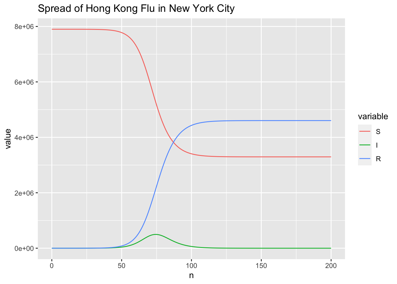
For the spread dynamic of the disease, I am interested in the time \(t\_{max}\) when the number of infected people gets maximum and the corresponding maximum number of infected people \(I\_{max}\). \(t\_{max}\) and \(I\_{max}\) are also key measures to evaluate the performance of the absolute humidity-driven SIRS model in
Yang et al. (2014). The following codes give \(t_{max}\) and \(I_{max}\).
which.max(r$I)
## [1] 75
max(r$I)
## [1] 497473.6
Comparing to the results of the study case
The SIR Model for Spread of Disease, the trends of \(S(t)\), \(I(t)\) and \(R(t)\) curves are correct. Furthermore, \(t_{max} = 75\) is the same to the approximate value of 75 identified from the figure.
1.3 RK4SIR.Yang function
Based on the propagateParSIR function from the code shipping with
Yang et al. (2014), I just reproduce the algorithm for easily understanding and create the following function RK4SIR.Yang to solve the SIR model.
RK4SIR.Yang <- function(n, beta, gamma, S0, I0, R0 = 0, dt = 1) {
  N <<- S0 + I0 + R0  # fixed population

  S <- c(S0, rep(0, n))
  I <- c(I0, rep(0, n))
  R <- c(R0, rep(0, n))
  for (i in 1:n) {
    Si <- S[i]
    Ii <- I[i]
    S.k1 <- dSdt(i, Si, Ii)
    I.k1 <- dIdt(i, Si, Ii)

    Ts1 <- Si + dt / 2 * S.k1
    Ti1 <- Ii + dt / 2 * I.k1
    S.k2 <- dSdt(i + dt / 2, Ts1, Ti1)
    I.k2 <- dIdt(i + dt / 2, Ts1, Ti1)

    Ts2 <- Ts1 + dt / 2 * S.k2
    Ti2 <- Ti1 + dt / 2 * I.k2
    S.k3 <- dSdt(i + dt / 2, Ts2, Ti2)
    I.k3 <- dIdt(i + dt / 2, Ts2, Ti2)

    Ts3 <- Ts2 + dt * S.k3
    Ti3 <- Ti2 + dt * I.k3
    S.k4 <- dSdt(i + dt, Ts3, Ti3)
    I.k4 <- dIdt(i + dt, Ts3, Ti3)

    S[i + 1] <- Si + dt / 6 * (S.k1 + 2 * S.k2 + 2 * S.k3 + S.k4)
    I[i + 1] <- Ii + dt / 6 * (I.k1 + 2 * I.k2 + 2 * I.k3 + I.k4)
    R[i + 1] <- N - S[i + 1] - I[i + 1]
  }
  return(data.frame(n = 0:n, S = S, I = I, R = R))
}
Note that RK4SIR.Yang is a bit different from RK4SIR in calculating \(k_1\), \(k_2\), \(k_3\) and \(k_4\). The functionality of RK4SIR.Yang is also tested by the same case.
Call RK4SIR.Yang to simulate the spread of Hong Kong flu in New York city.
r <- RK4SIR.Yang(n, beta, gamma, S0, I0)
Plot \(S(t)\), \(I(t)\) and \(R(t)\) curves.
r.plot <- melt(r, id = "n", measure = c("S", "I", "R"))
p <- ggplot(r.plot, aes(x = n, y = value, group = variable, color = variable))
p + geom_line() +
  ggtitle("Spread of Hong Kong Flu in New York City")
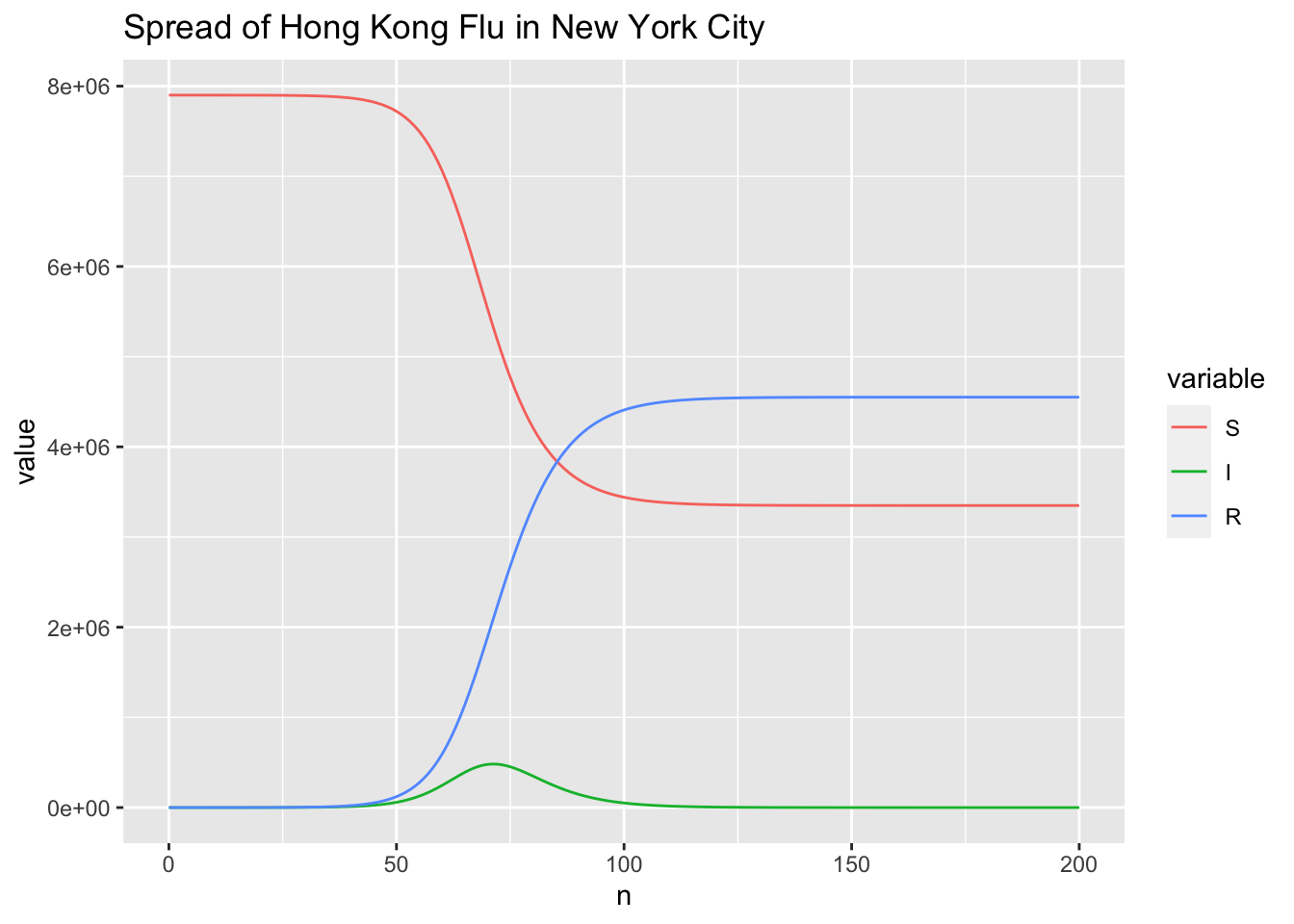
Extract \(t_{max}\) and \(I_{max}\).
which.max(r$I)
## [1] 72
max(r$I)
## [1] 482429.6
Comparing to the results of RK4SIR, the results of RK4SIR.Yang show that the infected indiviuals reaching peak is 3 days earlier and the number of infected individuals is more than 15,000 less. I doubt the RK4SIR.Yang function gives a wrong solution. To figure out which function (RK4SIR or RK4SIR.Yang) implements the RK4 method correctly, I also solve the SIR model by directly calling ODE solvers from the existing software package, including deSolve package and MATLAB.
1.4 deSolve package
deSolve package provides general solvers for inital value problems of ODE, PDE, DAE and DDE. rk4 function from deSolve package is an implementation of the classical RK4 integration algorithm. The steps of invoking rk4 function to solve the SIR model are as follows.
Firstly, define the initial values and parameters used in the SIR model.
# initial (state) values for SIR model
y0 <- c(S = S0, I = I0, R = 0)
# vector of time steps
times <- 0:n
# vector of parameters used in SIR model
params <- c(beta = beta, gamma = gamma)
Secondly, define the SIR model.
SIR <- function(t, y, params) {
  with(as.list(c(params, y)), {
    dS <- -beta * S * I / N
    dI <- beta * S * I / N - gamma * I
    dR <- gamma * I
    list(c(dS, dI, dR))
  })
}
Last, call rk4 function to solve the SIR model and plot the results.
library(deSolve)
r <-  rk4(y0, times, SIR, params)
plot(r)
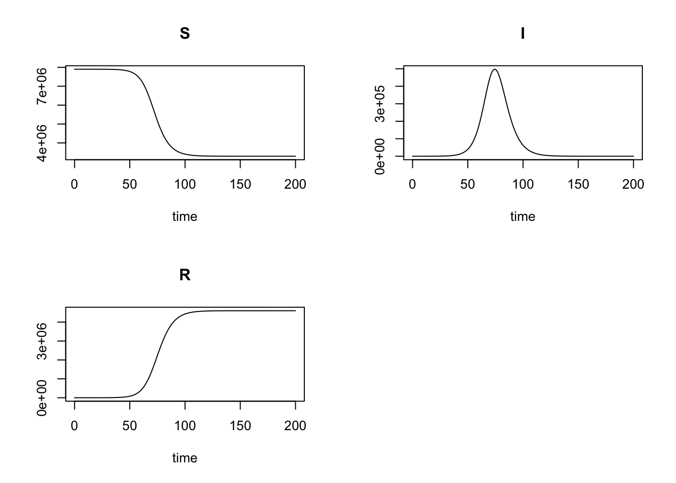
Similarly, extract \(t_{max}\) and \(I_{max}\).
which.max(r[, "I"])
## [1] 75
max(r[, "I"])
## [1] 497473.6
The results are the same to those of RK4SIR function. As deSolve is a mature package and has been used by numerous users, I believe the \(t_{max} = 75\) and \(I_{max} = 4.97474\times 10^{5}\) given by RK4SIR function are correct.
1.5 ode45 function
Furthermore, I solve the SIR model by calling ode45 function from MATLAB to further confirm my judgement. The codes are organized in two MATLAB scripts SIR.m and simSIR.m. Since the whole process is very similar to the R code, I would not explain the codes in detail. Here, I just present the codes.
SIR.m defines the ODEs of the SIR model.
function dy = SIR(t, y, beta, gamma, N)
% only two ODEs of SIR model are independent
% solving three ODE together, MATLAB gives wrong solution
S = y(1);
I = y(2);
dS = - beta * S * I / N;
dI = beta * S * I / N - gamma * I;
dy = [dS, dI]';
end
simSIR.m runs the specific simulation of the spread of Hong Kong flu in New York city and gives the results of interest.
clear

t = 0:200;
S0 = 7900000;
I0 = 10;
R0 = 0;
N = S0 + I0 + R0;
y0 = [S0, I0];
beta = 1 / 2;
gamma = 1 / 3;
options = [];

[T, Y] = ode45(@SIR, t, y0, options, beta, gamma, N);
% plot S, I, R curves
S = Y(:, 1);
I = Y(:, 2);
R = N - S - I;
plot(T, S, '-r', T, I, '-g', T, R, '-b')
title('Spread of Hong Kong Flu in New York City')
xlabel('Days')
ylabel('Value')
legend('S','I', 'R')

% peak of the infected
[maxVal, ind] = max(Y(:, 2))
% add veritical line to indicate the peak
ylim = get(gca, 'ylim');  %  get y range
hold on
plot([ind - 1, ind - 1], [ylim(1), ylim(2)], 'LineStyle', '--')
The results of running simSIR.m are
>> simSIR

ind =

    75

maxVal =

   4.9755e+05

Note that by default MATLAB’s ode45 solver is
Dormand–Prince method (alias dopri5), which is also a member of the Runge–Kutta family of ODE solvers. As ode45 is adaptive stepsize integration algorithm, it can give more accurate numerical solution than RK4 method.
rk45dp7 (alias ode45) method from deSolve package provides ode45 solver for ODEs in R. Solve the SIR model by using ode45 method in deSolve and extract \(t_{max}\) and \(I_{max}\).
r <-  ode(y0, times, SIR, params, method = rkMethod("ode45"))
# peak of the infected
which.max(r[, "I"])
## [1] 75
max(r[, "I"])
## [1] 497474.2
\(I_{max}\) given by rk4 and ode45 from deSolve package are almost the same, but both are approximate 80 less than that of ode45 in MATLAB. The results of ode45 provided by R and MATLAB are both right as the discrepancy results from the inherent difference in numerical precision between R and MATLAB. For more details refer to
the post.
The results given by both deSolve package and MATLAB show that \(I_{max} = 75\) is the right answer. I am pretty sure that the results from RK4SIR function are correct; however, the RK4SIR.Yang function \({\color{red}{doesn't\ correctly}}\) implement RK4 method for solving SIR model. Since the RK4SIR.Yang function gives a bit ealier \(I_{max}\), I wonder whether this wrong RK4 method has any influence on the conclusions of
Yang et al. (2014)
2 Incidence
2.1 Preliminary
Instead of \(S(t)\), \(I(t)\) and \(R(t)\) of SIR model, health workers in practice often collect daily number of newly infected people. This is the loosely expressed
incidence. Besides incidence, cummulative incidence is also of interest. Let \(C(t)\) denote incidence at time \(t\), \(P(t)\) denote cummulative incidence at time \(t\). \(C(t)\) and \(P(t)\) can be calculated as follows
$$
\begin{aligned}
& C(t) = \frac{dP}{dt} = \frac{\beta SI}{N} \\
& C(t_0) = S_0 \\
& P(t) = \int_0^t{C(t)}dt = \int_0^t{\frac{\beta SI}{N}}dt
\end{aligned}
$$
In some references,
cummulative incidence (also known as incidence proportion) refers to the number of new cases \(P(T)\) within a specified time period \(T\) divided by the size of the population initially at risk \(N\), expressed as \(P(T)\) cases per \(N\) persons, or \(\frac{P(T)}{N}\times 100\%\). The rigorous definition of incidence is
incidence rate, which is expressed as \(P(T)\) cases per \(N\) persons per \(T\) time, or \(\frac{P(T)}{N\times T}\times 100\%\).
2.2 RK4SIR function
A logical parameter incidence is added to RK4SIR function to control whether or not incidence and cummulative incidence are returned.
RK4SIR <- function(n, beta, gamma, S0, I0, R0 = 0, dt = 1, incidence = FALSE) {
  N <<- S0 + I0 + R0

  S <- c(S0, rep(0, n))
  I <- c(I0, rep(0, n))
  R <- c(R0, rep(0, n))
  for (i in 1:n) {
    Si <- S[i]
    Ii <- I[i]

    S.k1 <- dSdt(i, Si, Ii)
    I.k1 <- dIdt(i, Si, Ii)

    S.k2 <- dSdt(i + dt / 2, Si + dt / 2 * S.k1, Ii + dt / 2 * I.k1)
    I.k2 <- dIdt(i + dt / 2, Si + dt / 2 * S.k1, Ii + dt / 2 * I.k1)

    S.k3 <- dSdt(i + dt / 2, Si + dt / 2 * S.k2, Ii + dt / 2 * I.k2)
    I.k3 <- dIdt(i + dt / 2, Si + dt / 2 * S.k2, Ii + dt / 2 * I.k2)

    S.k4 <- dSdt(i + dt, Si + dt * S.k3, Ii + dt * I.k3)
    I.k4 <- dIdt(i + dt, Si + dt * S.k3, Ii + dt * I.k3)

    S[i + 1] <- Si + dt / 6 * (S.k1 + 2 * S.k2 + 2 * S.k3 + S.k4)
    I[i + 1] <- Ii + dt / 6 * (I.k1 + 2 * I.k2 + 2 * I.k3 + I.k4)
  }
  R <- N - S - I

  if (!incidence) {
    return(data.frame(n = 0:n, S = S, I = I, R = R))
  } else {
    # newly infected per day (incidence)
    inc = c(I0, -diff(S))
    # cumulative incidence
    cum.inc = cumsum(inc)
    return(data.frame(n = 0:n, S = S, I = I, R = R, inc = inc, cum.inc = cum.inc))
  }
}
Use the updated RK4SIR function to track the time-varying incidence and cummulative incidence of the same study case.
r <- RK4SIR(n, beta, gamma, S0, I0, incidence = TRUE)
# # plot S, I, R, incidence, cummulative incidence curves
r.plot <- melt(r, id = "n", measure = c("S", "I", "R", "inc", "cum.inc"))
p <- ggplot(r.plot, aes(x = n, y = value, group = variable, color = variable))
p + geom_line() +
  scale_colour_discrete(name = "Legend",
                      breaks = c("S", "I", "R", "inc", "cum.inc"),
                      labels = c("Susceptible", "Infected ", "Recovered", "Incidence",
                               "Cummulative incidence")) +
  ggtitle("Spread of Hong Kong Flu in New York City")
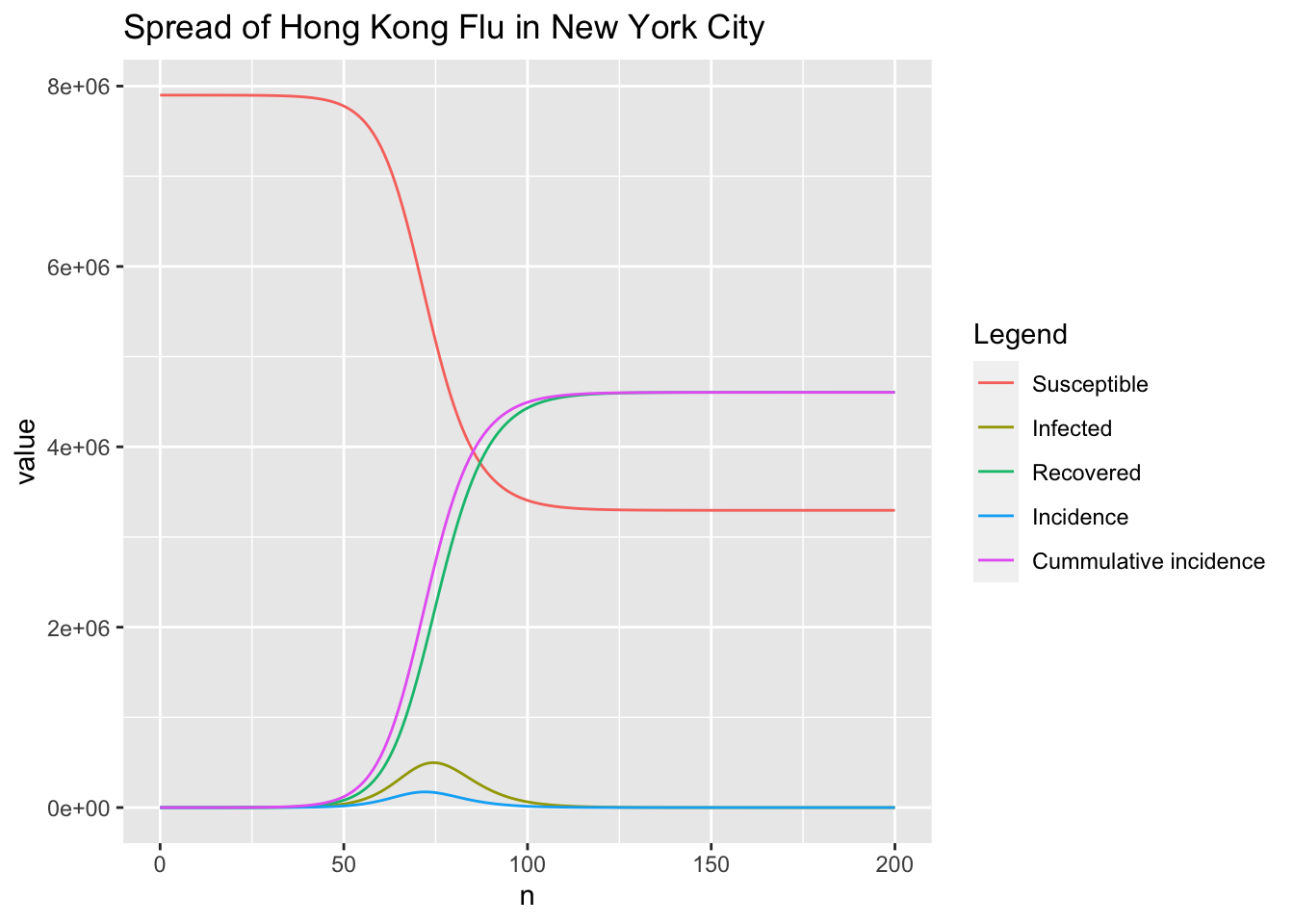
As shown in the above figure, the time when incidence reaches peak is a bit earlier than that of the infected people. The following codes give the exact results.
which.max(r$inc)
## [1] 73
max(r$inc)
## [1] 173488.5
2.3 RK4SIR.Yang function
I also update RK4SIR.Yang function to return cummulative incidence based on the algorithm from propagateParSIR function. The initial cummulative incidence \(C_0\) is 0, which is \(S_0\) in RK4SIR function; however, I think it’s more consistent to set \(C_0 = S_0\). Notably, the RK4 method for RK4SIR.Yang hasn’t been corrected and the function doesn’t return incidence.
RK4SIR.Yang <- function(n, beta, gamma, S0, I0, R0 = 0, dt = 1, incidence = FALSE) {
  N <<- S0 + I0 + R0

  S <- c(S0, rep(0, n))
  I <- c(I0, rep(0, n))
  R <- c(R0, rep(0, n))
  cum.inc <- rep(0, n + 1)  # cumulative incidence
  for (i in 1:n) {
    Si <- S[i]
    Ii <- I[i]
    S.k1 <- dSdt(i, Si, Ii)
    I.k1 <- dIdt(i, Si, Ii)
    CI.k1 <- -S.k1

    Ts1 <- Si + dt / 2 * S.k1
    Ti1 <- Ii + dt / 2 * I.k1
    S.k2 <- dSdt(i + dt / 2, Ts1, Ti1)
    I.k2 <- dIdt(i + dt / 2, Ts1, Ti1)
    CI.k2 <- -S.k2

    Ts2 <- Ts1 + dt / 2 * S.k2
    Ti2 <- Ti1 + dt / 2 * I.k2
    S.k3 <- dSdt(i + dt / 2, Ts2, Ti2)
    I.k3 <- dIdt(i + dt / 2, Ts2, Ti2)
    CI.k3 <- -S.k3

    Ts3 <- Ts2 + dt * S.k3
    Ti3 <- Ti2 + dt * I.k3
    S.k4 <- dSdt(i + dt, Ts3, Ti3)
    I.k4 <- dIdt(i + dt, Ts3, Ti3)
    CI.k4 <- -S.k4

    S[i + 1] <- Si + dt / 6 * (S.k1 + 2 * S.k2 + 2 * S.k3 + S.k4)
    I[i + 1] <- Ii + dt / 6 * (I.k1 + 2 * I.k2 + 2 * I.k3 + I.k4)
    R[i + 1] <- N - S[i + 1] - I[i + 1]
    cum.inc[i + 1] <- cum.inc[i] + dt / 6 * (CI.k1 + 2 * CI.k2 + 2 * CI.k3 + CI.k4)
  }
  if (!incidence) {
    return(data.frame(n = 0:n, S = S, I = I, R = R))
  } else {
    return(data.frame(n = 0:n, S = S, I = I, R = R, cum.inc = cum.inc))
  }
}
2.4 Benchmark
microbenchmark package is a good option for benchmarking functions. I use microbenchmark function to compare rk4, RK4SIR and RK4SIR.Yang 1000 times.
library(microbenchmark)
compare <- microbenchmark(rk4(y0, times, SIR, params),
                          RK4SIR(n, beta, gamma, S0, I0, incidence = TRUE),
                          RK4SIR.Yang(n, beta, gamma, S0, I0, incidence = TRUE),
                          times = 10)
# change expr for plot
compare$expr <- gsub("rk4(y0, times, SIR, params)", "rk4",
                     compare$expr, fixed = TRUE)
compare$expr <- gsub("RK4SIR(n, beta, gamma, S0, I0, incidence = TRUE)", "RK4SIR",
                     compare$expr, fixed = TRUE)
compare$expr <- gsub("RK4SIR.Yang(n, beta, gamma, S0, I0, incidence = TRUE)",
                     "RK4SIR.Yang", compare$expr, fixed = TRUE)
compare
## Unit: milliseconds
##         expr       min        lq      mean    median        uq       max neval
##          rk4 10.522828 10.849218 12.314321 11.330950 14.672388 15.626585    10
##       RK4SIR  1.691710  2.008025  2.244679  2.157010  2.655575  2.672397    10
##  RK4SIR.Yang  1.627021  1.879434  6.647515  2.081856  2.122347 48.506175    10
Draw a comparison of distribution times.
p <- autoplot(compare)
## Coordinate system already present. Adding new coordinate system, which will
## replace the existing one.
p + geom_violin(aes(color = expr, fill = expr)) +
  theme(legend.position = "none")
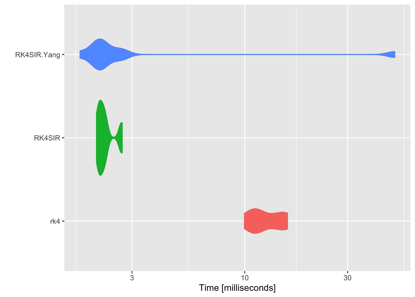
rk4 function from deSolve package runs much slower than both RK4SIR and RK4SIR.Yang fucntions as it takes much time to spin up for calling external FORTRAN or C functions. Though RK4SIR function performs the extra calculation of incidence, the benchmarking results show that RK4SIR function still runs faster than RK4SIR.Yang function. This is because RK4SIR.Yang function calculates cummulative incidence one by one per iterative formula while RK4SIR function directly apply diff function to the resulting vector S to accomplish the calculation. diff function is a vector operation and takes much less time.